Bottom-up synthesis of Density Functional Theory (DFT)

From the Born-Oppenheimer approximation to the Kohn & Sham equation.

💪 Motivation

“Today we know less than 1% of known compounds in the world; less than 1% of the materials properties.”

Gerbrand Ceder @ The Material Desing Revolution the World Economic Forum (2014, Davoz).

1. Introduction

Go to TOC

Definition:

A mathematical model about a sufficiently large set of natural phenomena is called an “ab initio model ” or a “first principles model” if the starting point of the model can not be further reduced to more fundamental concepts (at least not within the language of the considered natural phenomena).

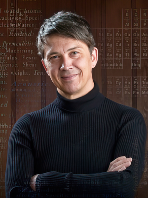
By Pr. Stefaan Cottenier @ Ghent University.

Furhtermore, the main idea is to tame the following beast:

Where the Hamiltonian is given in atomic unit for \(N_e\) electrons and \(N_n\) nucleus as following:

The right-hand side of \((2)\) are respectively: electron and nucleus kinetic energy, electron-electron and nuclei-nuclie Coulomb interaction and the electron-nuclie Coulomb interaction.

2. How to tame Schrödinger equation ?

Go to TOC

2.1 Born-Oppenheimer approximation

The basic idea is the following: ”We consider the nuclei as stationary objects, so we freeze the nuclear positions.”. We say that this approximation is adiabatic (We move from \(4(Ne + Nn) \longrightarrow 4Ne\)).

The previous wavefunction should be anti-symmetric. The problem is reduced into solving the Schrödinger equation for the following Hamiltonian:

ℹ️ Note: that \(\textbf{BO}\)-approximation is a major simplification, but it is way too hard to solve! more work is needed.

2.2 Hartree-Fock method (post-HF method)

Go to TOC

💡 The main idea:
For all the possible sets of the wavefunctions that can describe our system, we search for the one associated to the ground state. With the following restrictions:

• Just the anti-symmetric wavefunctions;

• Use Salter determinant;

• The energy minimization principal.

⚠️ At the end this is an approximation (work well for chemistry topics, not for solids).

The first step is visualizing the terms in the reduced Schrödinger equation after \(\textbf{BO}\) approximation. After all, we end up with:

Notice that we omitted the constant term, the reason will be more obvious in the following derivations. The Hartree-Fock method is a variational, wavefunction-based approach. Although it is a many-body technique, the approach followed is that of a single-particle picture, i.e. the electrons are considered as occupying single-particle orbitals making up the wavefunction. Each electron feels the presence of the other electrons indirectly through an effective potential. Each orbital, thus, is affected by the presence of electrons in other orbitals. Now to build our wavefunction, instinctively we write our function as the product of the orbitals occupied by the electrons, and for simplicity we drop the spin degrees of freedom:

❗ But wait, this expression violate the first restriction mentioned above ! We need another tools that respect the anti-symmetric feature of the wavefunction.

2.2.1 Slater expression

Go to TOC

One way to overcome the raised problem is the so called \(Slater\) determinant:

Now, we will try to write more compact formula for our wavefuction:

2.2.2 Energy minimization

Go to TOC

As the \(\textbf{HF}\) method relies on a variational principal:

We start by evaluating the expected value of the single particle (first term on the right side ):

The trick that works with me is to write down \(\textcolor{green}{first}\) the orbitals that the Hamiltonian is mainly! applied on. Then we write the remaining terms as single \(bra-ket\) products :

With the \(anzats\): \(\langle\varphi_j|\varphi_i\rangle=\delta_{ij}\)

Since we end up with one sum(\(i=j\)) \(N!\) times over all the orbitals, we have always the same \(+\) sign in front of the product:

In conclusion the first term in \(\textbf{HF}\) energy is the expected total energy of all the single particles treated individually.

Let’s tackle the second terms:

We use the same tricks as before:

Which is reduced into ( Notice the order \(n < m\).):

Here we have one permutation operators \(P\) acting on the order of the set of orbitals \(\{1, 2, \dots, n, \dots, m, \dots, N\}\). It is not obvious, but clearly we are expecting something to pop-up for sure! And the idea is to separate all the \(even\) and the \(odd\) permutations in the previous set:

For both \(even\) or \(odd\) terms we have \(N!\) times repeated quantities. Hence we find:

At the end we get the following expression for our many-body problem:

2.2.3 Hartree-Fock equation

Go to TOC

In this section we will apply the variational principale on the last equation and the aim is to minimize the total energy:

We use the Lagrange multipliers and the orthogonality of the set of our wvefunctions basis as following:

The \(F\) stand for \(Fock\) operator in the last equation. Now we will consider small change in our wavefunction basis (\(\varphi \longrightarrow \varphi + \delta \varphi\)). We first treat the the term with the \(Langrange\) multipliers:

We can write the second term as:

We move forward to differentiate the single electrons expectation value:

Since \(\hat{h}_1\) is hermitian operator i.e \(\left(\hat{h}_1\right)^{\dagger}=\hat{h}_1\):

Where \(C.C\) stand for \(Complex\ Conjugate\). Then we work with second term of \(Hartree-Fock\) energy (\(E_{HF}\)), step by step we will start by the electrons coulomb interaction:

We notice that we have \(C.C\) that pop-up automatically as in the previous treatment:

After this we are arrive to the exchange term, and with the same treatment:

I highlighted the corresponding lines to show the trick!

Since \(\{r_i;r_j\}\) are \(dummy\) variables, the integral value doesn’t change if we swap the indices. Also, the operator \(\hat{h}_2\) is invariant by changing the order (\(\hat{h}_2\) represent a coulomb interaction ):

Hence, we can write in more condensed way as before:

Now we will omit the notation \(\varphi_i(r_j)\) :

We are almost there! Lets write all the terms:

It is not obvious, and the following argument that I rise here may be naive! but the factor of half disappear. Why? We can justify it by the interchanging the indices \(i\ \&\ j\) order, or we say at some point of the summation; the states are reached twice! At this point, it is more proper and urgent! to write the last equation in its integral form:

Now we have our final \(action\) expression (\(F\)) of our system, we take the derivative of \(F\) with respect to some \(k^{th}\) bra (\(\bra{\delta\varphi_k} \equiv \varphi^*_k\)). Notice that \(\frac{\delta C.C}{\delta\varphi} = 0\) (the reason for choosing the \(bra\) over the \(ket\) will be obvious at the end!).

The idea of factoring the \(ket\) is just to re-write our expression in Schrodinger-equation like form, and it’s not rigorous from the mathematical point of view! Hence, Factoring out the \(\ket{\varphi_k}\) gives:

Now we can go back to \(bra-ket\) notation without confusion:

This is the why we choose \(bra\) over \(ket\), to end-up with system of Schrodinger-like equations! for which \(\hat{J}_i\) is an integral operator stand for the classical interaction of an electron distributions given by \(|\varphi_j|^2\) and is called the \(\textbf{direct\ term}\). While \(\hat{K}_j\) called the \(\textbf{exchange operator}\), has no classical analogue and it is a direct result of the antisymmetry property of the wavefunction. The Fock operator is given by:

The problem is reduced into finding the eigenvalues of the following set of equations:

For which the solutions \(\varepsilon_k\) hold the new identity of the Lagrange multipliers.

2.2.4 KOOPMAN’S THEOREM & The Ionization energy

Go to TOC

In this section we use \(Koopman's\ theorem\) to give an insight interpretation to the eigenenergies \(\varepsilon_k$\) we find in the previous equation. We will consider two system with (N-1) and N electrons respectively. For which the system of \(N-1\) electron is missing one electron on some orbital “n”. Also, beside omitting the spin orbitals degrees of freedom, we postulate that the orbitals are unchanged during this process. We start by writing the HF energy of both system:

Notice that for first line we do not have the “n” orbital in our sum. Now, we evaluate the difference \(E_{HF}^{N-1}-E_{HF}^{N}\) term by term through the full expansion of both summations:

Since the indices \(k\) and \(j\) are irrelevant (\(k\equiv j\)), and by make use of the identity \(\bra{f_1f_2}\hat{A}\ket{f_3f_4} = \bra{f_2f_1}\hat{A}\ket{f_4f_3}\), we get:

The last equation is nothing less that the negative eigenenergy of the \(\textbf{Fock}\) operator on the orbital “n”:

2.2.5 Hartree-Fock-Roothaan

Go to TOC

One of the attempt to solve the \(\textbf{HF}\) equation was done in 1951 by \(\textbf{Roothaan}\). Clemens C. J. Roothaan was a Dutch physicist and chemist known for his development of the self-consistent field theory of molecular structure². For a quick read brows the Roothaan equation .

²: Wikipedia-Bibliography

3 The many-body Problem as electron density dependence

Go to TOC

In this section we will rewrite the Hamiltonian as function of the electron density. Again we will treat the Hamiltonian as a spin-less problem. This is the core idea behind density dunctional theory where the function we are interested in take another function and return an output a.k.a number (\(f \longrightarrow I[f]\)).

But first we need to write the later entity \(n(r)\). So to start we define \(n(r_1)\) the electron density of finding an electron at position \(r_1\) while the rest of electrons set are at positions \(\{r_2,r_3, \dots, r_N\}\) as following:

First thing to notice is that we can write the product of the \(bra-ket\) function as the norm squared \(|\Psi(r_1, r_2, \dots, r_N)|^2\) (the operator \(\hat{n}(r_1)\) does not acts on the wavefunction) which yields:

By following the same reasoning the electron density of many-body system \(n(r)\) is given by the sum of all individual electrons densities(the definition \(n(r)= \sum_i^N n(r_i)\), is justified by seeing the operator of \(\hat{n}(r)\) as a linear one):

Since the propriety of the Norm squared of the wavefunction does not change with its arguments shuffled(\(|\Psi(r_1, \dots r_i,r_j,\dots, r_N)|^2 = |\Psi(r_1, \dots r_j,r_i,\dots, r_N)|^2\)). It is obvious that we end-up having \(N\) equal terms, because of the indistinguishable nature of electrons:

If we integrate the last equation over the remaining spaces we get the electrons number(here we consider a normalized wavefunction):

3.1 The electrons-ions interaction

Go to TOC

Previously we had established the electrons-ions interaction, now we will introduce the electrons density \(n(r)\). We start as always by taking the expectation values of the later coulomb interaction:

The operator \(\hat{V}_{e-n}\) allows for the appearance of the Norm squared of the wavefunction. Then we expand the summation over the electrons:

The factor of each individual coulomb interaction integral is the same! Beside the same trick of shuffling the arguments and changing re-arranging the indices, we use the dummy variables \(r_i \longrightarrow r\) we rewrite:

We notice the appearance of the electron density that we define it previously, hence:

3.2 The electrons-electrons interaction

Go to TOC

Using the same manner that we did in the last section we will introduce the electron density. Note that it is not quite the same quantity \(n(r)\)! Within the electrons-electrons interaction. And the starting point is always the avearage value:

We will expend over the \(i\) summation:

Lets expand the first term over the summation \(j\neq i\):

We apply a dummy variable changing \(r_1\longrightarrow r\) and \(r_j\longrightarrow r'\):

Basically the integral over the \(\mathbb{R}^{3(N-2)}\) space is the same, and we have \((N-1)\) term. And again the shuffling propriety of the wave function:

We treat each \(N\) remaining term the same, and we get:

Now we define the new pair electron density as following:

Finally the electrons-electrons interaction is reduced into:

Here we will re-write the new raised quantity as an expansion of the usual density:

Which lead to:

The \(E_c\) is a correction term.

3.3 The Kinetic Energy

Go to TOC

Yet, we did not write our Energy as a functional of the density \(n(r)\). We still have the Kinetic term which is hard to deal with since we have the operator \(\nabla^2\) that act on the wavefunction (\(\Psi\)). In order to tackle the kinetic energy, we make one of the key assumptions of density functional theory. We assume that the density can be written as the sum norm squares of a collection of single-particle orbitals:

These orbitals are called \(\textbf{Kohn-Sham orbitals}\) and they are initially completely unspecified in much the same way as in the orbitals in the Slater determinant in the \(\textbf{Hartree-Fock}\) formalism. The above form cannot really be considered an approximation. It simply says that instead of the full many-particle system we consider an auxiliary system of single-particle orbitals that have the same ground state density as the real system. Hence the Kinetic energy can be written in term to the KS orbitals to a correction term; as following:

3.4 Introducing the Exchange Correlation term

Go to TOC

In the following we will refer to the paper of \(\textsc{Kohn and Sham}\)³. As it was reported in the later paper, the ground state energy has the following form:

Where:

Where \(\varepsilon_{xc}\) is the exchange and correrrelation energy rep electron of a uniform electron gas of density \(n(r)\)³.

The origin of this term is the difference between a system of N interacting and noninteracting particles. More specifically:

• \(\textbf{Exchange}\) energy is the Pauli repulsion, omitted in the Hartree term;
• \(\textbf{Correlation}\) energy is the repulsion between electrons.

³ Walter Kohn and Lu Jeu Sham. Self-consistent equations including exchange and correlation effects. Physical review, 140(4A):A1133, 1965

3.5 THE HOHENBERG-KOHN THEOREM

Go to TOC

Theorem I:

Proof

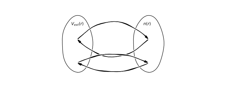
Let assume that exist two different external potential \(V_{ext}^{(1)}(r)\) and \(V_{ext}^{(2)}(r)\) that gives rise to the same electrons density for non-degenerate ground state \(n(r)\). Hence, we have two wavefunction for two Hamiltonian:

In the other hand:

Which is a \(\textbf{Contradiction}!!!\)

Theorem II:

Proof:

Let \(E\) be the exact energy of the ground state of our system of \(N\) interacting electron (non-degenerate state), then:

Where \(G[n(r)]\) is a universal function of the density:

4 Kohn and Sham Equation: Derivation attempt!

Go to TOC

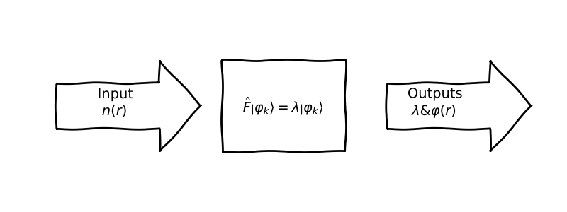
We will try to re-derive the \(\textbf{KS}\) equation by following the same procedures used in \(\textbf{HF}\) approach. The idea is as simple as the minimization over the wavefunction! But an approximation is needed. As we discussed previously we already write the Energy as functional of the density (i.e: \(E[n(r)]\)); but it was shown that the kinetic energy raise a problem, that it can not be written in terms of the density \(n(r)\), so we consider the \(\textbf{KS}\) orbitals that builds the density from ground i.e: \(n(r)=\sum_i^N |\varphi(r)|^2\), hence the kinetic term can be minimized through the set of these orbitals! that we postulate theirs orthogonality constraints:

Where \(\varepsilon\) stand for the \(\textbf{Lagrange multiplier}\). The two first terms on the left hand side are easy to manipulate!

We will try to tackle the universal function \(G[n]\):

For the \(\textbf{Lagrange multiplier}\) we get:

The final expression called \(\textbf{KS-equation}\) has the foollowing form:

Which is reduced into:

The problem is now can be solved exactly if we know the function \(V_{xc}=\frac{\delta E_{xc}[n(r)]}{\delta n(r)}\)!

5 Solving KS equation

Go to TOC

In this section we will see how we can solve \(\textbf{KS-equation}\), but first we will write down the matrix formula equivalent to the Schrodinger-like equation; using the Planewave expansion. Without further ado, we start by defining our wavefunction (i.e: the \(\textbf{KS-orbitals}\)) as following:

Where, \(\Omega\) is the volume of the real space where we are working in, and \(c_{i,q}\) are the Fourier coefficients of the wavefunction. Note, that we are moving to the reciprocal space \({\overrightarrow{q}}\) instead of the real one, which will make \(\textbf{Fourier transform}\) the pillars of this work! For our Hamiltonian that is described by \(\textbf{KS}\) equation will be rewritten as follwing:

Where, \(\hat{T}_{s}\) is the single-particle kinetic energy and \(\hat{V}_{eff}\). Where \(\hat{V}_{eff} = \hat{\Theta} + \hat{V}_{xc}\). Is the effective potential which contains the external, \(\textbf{Hartree}\) (i.e: \(\hat{\Theta}\)) and \(\textbf{exchange-correlation}\) (i.e: \(\hat{V}_{xc}\)) parts. So far we can write the wavefunction in the basis set of \(\{\overrightarrow{q}\}\) as following:

Now to get the eigenvalues \(\varepsilon_i\) we evaluate the following product:

Which yield to :

where \(\underline{\underline{H}}\) is the Hamiltonian in matrix representation and \(\underline{\underline{C}}\) is a vector of coefficients. Now, we will work out the kinetic energy term:

In the planewave representation, the kinetic energy term assumes an extremely simple, diagonal form. Now we proceed with effective potential, since \(V_{eff}\) has the periodicity of the lattice and therefore the only allowed Fourier components are those with the wavevectors in the reciprocal space of the crystal:

Performing the same product as previously gives:

By make use of the change in variable, by make \(\overrightarrow{q} = \overrightarrow{k}+\overrightarrow{G}_m\) and \(\overrightarrow{q'} = \overrightarrow{k}+\overrightarrow{G}_m'\), so the wave vectors (\(q\ \&\ q'\)) differ by a reciprocal lattice vector. which brings the Schrodinger-equation like to the \(k\) space:

In summary, we reduced the problem into the First \(\textbf{Brillouin zone}\) (The primitive cell in the reciprocal space), thanks to \(\textbf{Bloch's theorem}\). Now it is important to see how the \(V_{eff}\) can be written in the \textbf{Fourier Space}. For the sake of notation we denote \(n(\overrightarrow{r})\) the real electron density and \(\rho(\overrightarrow{G})\) it conjugate in the reciprocal space.

5.1 The electron-electron interaction (Hartee Energy term)

Go to TOC

We use the same definition of the planewave expension for the electron density:

We write : \(\overrightarrow{u} = \overrightarrow{r}-\overrightarrow{r'} \longleftrightarrow d\overrightarrow{u} = \overrightarrow{r}\), and in the first exponential we add and subtract \(\overrightarrow{r'}\):

We separate the independent integral and write \(\underset{\mathbb{R}^3}{\int d\overrightarrow{u}} =2\pi\int_{0}^{\infty}\int_{0}^{\pi} u^2 du sin(\theta) d\theta\):

The last integral factor it is not a proper integral!

Rigorously the limit does not exist (not unique a.k.a \(\lim_{x\longrightarrow a} f(x) \neq f(a) \))!

A further simplification: \(G = -\nu G'\), because the density is a physical measurable quantity, \(\mathcal{F}\{\Phi\}(\omega)=\mathcal{F}\{\Phi\}(-\omega)\), where \(\mathcal{F}\) is Fourier transform and \(\Phi\) physical entity i.e the negative and the positive frequency components are equal [see chapter 8 of Aschroft and Mermin’s “Solid State Physics”].

And by considering the propriety : \(\rho(\overrightarrow{G}) = \rho(\overrightarrow{G'})\)

5.2 The electron-electron interaction (Hartee Potential term) Go to TOC

With the same analogy:

And we ends up by having:

5.3 The exchange-correlation term

Go to TOC

As we have seen before that the last contribution of the effective potential in \(\textbf{KS}\) Hamiltonian is due to the change of exchange-correlation energy function over a small variation in the electron density (i.e: \(V_{xc}(\overrightarrow{r}) = \frac{\delta E[n(\overrightarrow{r})]}{\delta n(\overrightarrow{r})}\)). We will use the expression given by Walter Kohn et al. ³ for the later term, and since we can exchange the derivation of a function over the integral like the case with regular functions, note that we could derive first and perform the Fourier decomposition, and we ends up by having two terms:

³ Walter Kohn and Lu Jeu Sham. Self-consistent equations including exchange and correlation effects. Physical review, 140(4A):A1133, 1965

At this stage we shall say that we manage to perform Bottom-up synthesis of Density Functional Theory (DFT).

Thank you for reaching this points.